Detecting Melanoma Skin Cancer with Computer Vision

There were around 300,000 confirmed new cases of melanoma (malignant) skin cancer worldwide in 2018. During the same year, more than a million new non-melanoma (benign) cases were diagnosed. The numbers are most likely an underestimate due to various factors though (such as countries' lack of registries or wars).

The Scandinavian counties are all ranked very high in terms of cancer rates per capita, where Sweden, my home country, is ranked 6th, averaged over all sexes. A combination of white skin color and a society that considers being sun-tanned attractive likely contributes to these high numbers. Being able to quickly and accurately check a spot on the skin can thus be desirable for many. Using deep learning techniques and a publicly available dataset, we will test whether it's possible to classify melanoma from non-melanoma skin cancer using computer vision.

The dataset can be accessed on Kaggle through this link. There are in total 3,297 images, split into 2,110 train, 527 validation and 660 test images. It's a fairly small dataset, chosen specifically to save on computational costs. However, I will choose an implementation where the number of images can easily be scaled up to any number with practically no changes to the code.

The work will be documented in a Jupyter Notebook which can be hosted on a local machine or in the cloud. It's highly recommended to use a GPU as it will significantly speed up model training - perhaps by as as much as 10x. The dataset is small enough to be used with Google Colab (which has access to free GPUs that cover our requirements). The complete notebook can be accessed here.

Data processing and exploration

As with all other data related work we need to load and get to know the data before anything else. The images come in the size (224, 224) and I will keep them as is for now. If we run into problems with fitting the images into the GPU memory we might consider decreasing the resolution. We should be careful though as we might lose important information. Decreasing the batch size, which I initially set to 32, can be a safer alternative.

The data is stored in folders, one folder for the train set and one for the test set. Each one of those folders holds two other folders, one for each class - Malignant (1) and Benign (0). The validation set, used during training for checking the model performance to adjust the learning accordingly, will correspond to the last 20% of the data in the train folder.

We will create data generators that will feed the model during training with data in batches. By using batch training virtually any size of dataset can be processed during training and will allow us to scale up if needed. The generators also takes care of scaling the images from their original [0, 255] to a more suitable [0, 1] range for neural networks. This will allow faster convergence, and thus training, while also improving performance.

Running above code, we can confirm that we are dealing with a small dataset. 2110 images for training, 527 for validation and 660 for testing.

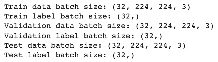
Additionally, we can do a quick sanity check on the three generators. We want the train data batches to have size (32, 224, 224, 3) while the labels should have size (32,). 32 refers to the batch size, while 224 and 224 to the image size and 3 to the image channel. Since we are working with color images, there should be one dimension for each RGB color.

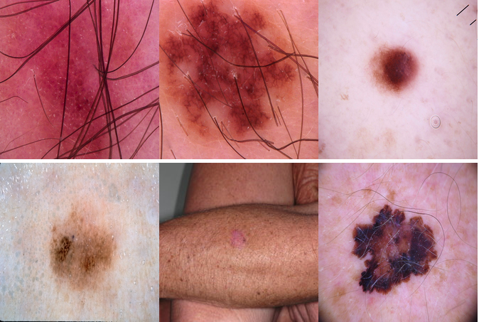
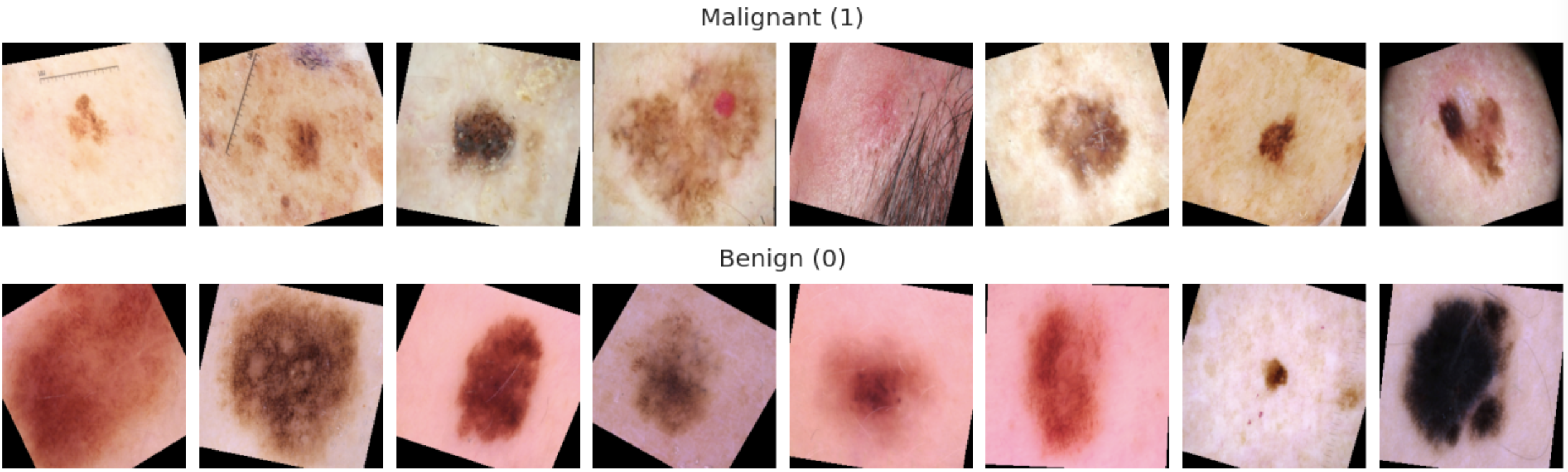
Next up, we will visualise some images by class to get a better understanding of what we are working with. These are all loaded from the train set.

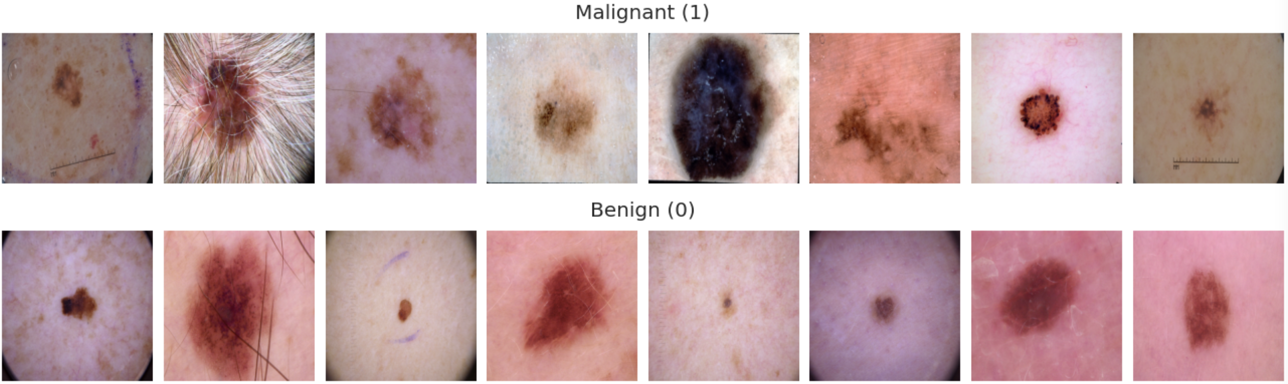
The malignant tumors (1), on average, do seem to look slightly uglier than the benign tumors (0), with some few exceptions. But it's a very difficult task for an untrained eye to distinguish between the upper and lower row, and I wouldn't feel confident trying to classify these on my own. Luckily we have radiologists, and perhaps also deep learning systems helping us out soon (in fact, these systems are already out there).

Let's continue by displaying the class ratio.

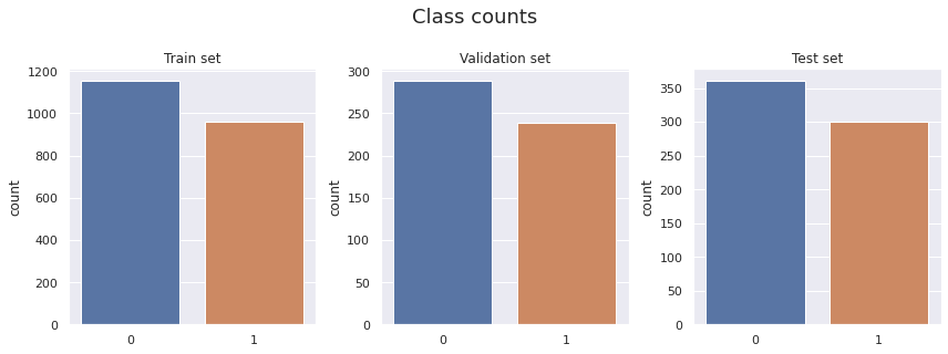
The class ratio is equal and there's little class imbalance to speak of with 55% benign images and 45% malignant across all three sets.

Next, define important metrics to keep track of during model training. We will optimise for AUC (because it represents a general better model) but keep a close eye on recall since it's worse to miss out on classifying a tumor as malignant than it is to accidentally classifying a benign as malignant. The former might lead to a patient's death while the latter, although very inconvenient, will only put the patient through more examinations.

Define initial bias and callbacks

Start by calculating the initial output bias. This will help the model to converge faster during training.

Callbacks can be used for several things in Keras. In this case we will implement:

• ModelCheckpoint: Used for storing the best model when evaluated on the validation set during training. We only save the best model, overwriting old models if the new is better.
• EarlyStopping: Deep learning model training takes time. This will cause training to stop if the validation AUC hasn't increased in 10 epochs.
• CSVLogger: Store the metrics after each epoch in a .csv file.

Baseline model

Neural networks are hard to train, with many knobs to tune in order to get the results you wish. For that reason, it's very easy to mess things up by introducing errors. A common approach, and one we will take here, is to start out with a simple model with few layers. This also has the inherit advantage of allowing us to find the most simplistic model for the problem that performs sufficiently well. We will try to adhere to the KISS principle.

SeparableConv2D layers will be used instead of the more common Conv2D layer since they are faster to train, require less memory, while often yielding superior results. MaxPooling2D layers are used to downsample the feature map after each convolutional layer and is chosen over other pooling alternatives due to their proven superior performance.

Since this is a binary classification problem, we add a fully connected classifier with a single output unit (Dense layer with 1 unit) and a sigmoid activation function in the output layer. The general purpose with activation functions is to enable mapping of non-linear relationships in the data.

A Relu activation function will be used in the hidden layers as it normally yield faster convergence compared with other alternatives. We also initiate the output bias we created above to better reflect the class imbalance in the dataset. That way the model doesn't have to spend time learning that during the first epochs. In this case though, the difference will be minimal as the classes are fairly well balanced.

The number of filters, the kerne_size, pool_size, Dropout rate, the number of hidden layers and the way they are stacked are all hyper parameters that should be tuned for optimal performance. Researchers are spending their entire PhDs on building these architectures which are later released to the public. We simply don't have that time to spend so we will go with something simpler. Later, we will make use of some of these architectures through Transfer Learning though - a very common approach in the field.

Create a baseline model

Create the baseline model using the previously defined make_base_model() function. Binary cross-entropy is used as loss function since this is a binary problem and because the target labels are stored in a vector, as we saw before (rather than one-hot encoded). Adam optimiser with default learning rate often works fine on problems like this.

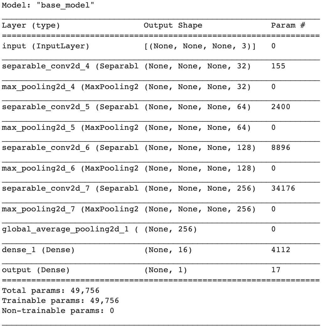
The resulting architecture has a total of 49,756 parameters, which are all trainable.

Train the model

Next up, we will train the model for 50 epochs and keep track of the resulting metrics on the train and validation sets. Store those in a variable called history. Note that because we implemented callbacks the model will stop training prior to 50 epochs if the validation AUC hasn't increased over 10 consecutive epochs.

Training will vary depending on the hardware we use, but by using a free K80 GPU on Google Colab it will take around 5 minutes.

Check training history

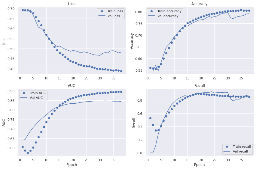
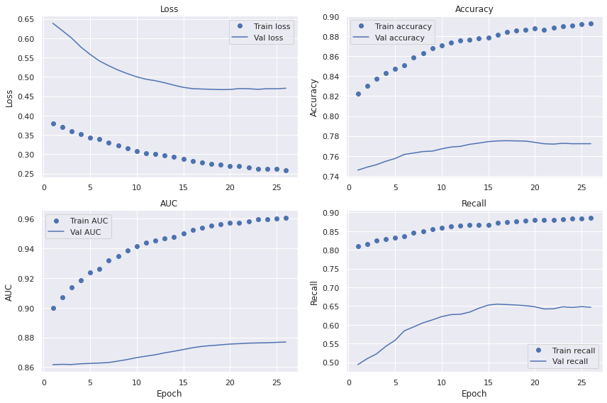
Plot the Loss, Accuracy, AUC and Recall for both the train and validation sets during training.

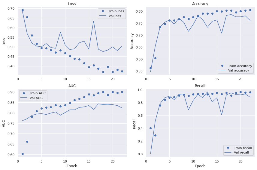
The first thing to note is how irregular the validation curves are with their zig-zag shape. We also note the high bias - in particular on accuracy. This is likely a result of the small model that is not able to learn the characteristics of the data properly. Variance is low with only minor differences between the train and validation curves across all metrics.

Ideally however, we would use something like Keras Tuner to properly build and evaluate an architecture like this. But as this is a very resource intensive process we will put it off for future work when using a more powerful GPU.

Plot confusion matrix

Let's evaluate the model on the test set. Remember that we stored only the best model during training, so we will use that. We will also plot a confusion matrix to better understand the model's strengths and weaknesses. The prediction threshold is set to 50%, meaning that the model needs to be at least 50% confident in order to classify a sample as malignant.

The model correctly classifies 295 malignant and 230 benign tumors. And it only misses out on 5 malignant tumors. So far so good. However, if we take a look at the number of benign tumors falsely being classified as malignant we see a serious problem. It seems that whenever the model is unsure of what class a sample belongs to it classifies it as malignant. Better safe than sorry one might think! But with 130 harmless tumors incorrectly classified as malignant many patients will face unnecessary worries and examinations. Clearly we can do better.

Plot the ROC and AUPRC

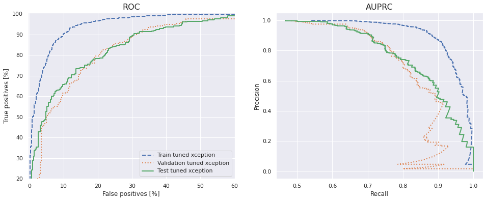
Before moving on though, let's plot the Receiver Operating Characteristic (ROC) and Area Under the interpolated Precision-Recall Curve (AUPRC). The curves are very useful as they display in a clear way the trade-off between true positives and false positives (as in the ROC) and precision and recall (as in the AUPRC); as one metric increase, the other one decreases. It's a common problem machine learning engineers and data scientists face.

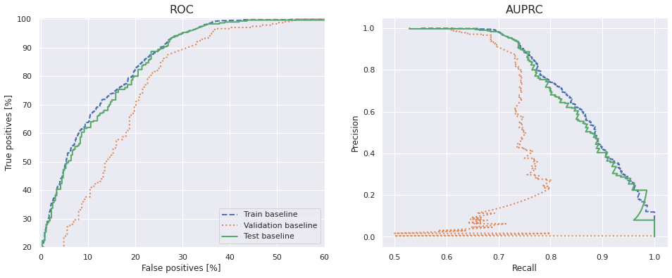
Ideally, the ROC should be as close up to the top left corner as possible while the AUPRC as high up to the right as possible. We can see that there's definitely room for improvement in both cases. The model is learning something though, and that's encouraging for coming steps.

Train and evaluate multiple baseline models

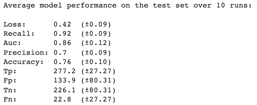
Due to randomness on both the system and TensorFlow level the results differ between each run (a run is here referred to building, training and evaluating a model). To get a better estimation of the model's performance, build, train and evaluate 10 models and average their results. Ideally, we would run even more models, but that would take very long time. For the purpose of this article, we can leave that for future work.

Start by defining a function that does all that for us and outputs the scores on the train, validation and test sets.

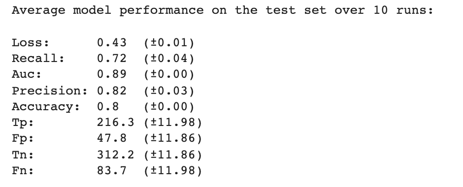
The results, with standard deviations, over 10 runs are displayed below. There are fairly large discrepancies between the lowest and highest values across all metrics (check the standard deviations within the parentheses). However, we can also see that already this fairly simple baseline model performs well with a Recall of 92%, AUC of 86% and Accuracy of 76%. Just as we pointed out before though, the precision is lower at 70% since the model seem to have a tendency of always predicting malignant when it's unsure.

Data augmentation

A common way of improving the performance of a model is to add more data. If that's not possible, then rotating, zooming, flipping, adjusting brightness and so fort on the data you already have, can often be a good and simple way of improving model performance. This is easily done in Keras using the ImageDataGenerator we used before. There are two large advantages of augmenting during data loading; we can take advantage of the parallel threads in the GPU, allowing faster processing as well as it makes the final production-ready model more robust by allowing it to take in any kind of raw images. That way we won't have to worry about correctly pre-processing the images in a parallel process as everything is taken care of by the model architecture.

Define data generators with augmentation

Rotation range is used to randomly rotate the images ±30 degrees while fill_mode='constant' fills out the discrepancy between the original and augmented image area with a constant value (black, or 0, in this case). Knowing that, the rest of the parameters are fairly self-explanatory.

Exactly how these parameters are set is something that can and should be experimented with for optimal model performance. Remember that with a larger specified range more new images will be created and the more time and processing power is needed to train the model. The advantage is that we can potentially get better results. Again, this is a common trade-off we often have to make.

The save_to_dir parameter for the train and validation generators are used to store the images processed by the generator. This is very useful for inspecting exactly what images are being fed into the model and can save us from a lot of headache if the model doesn't behave as expected. After repeated experimentation I have commented out these to save disk space.

Note that we do not use data augmentation on the validation and test sets as we don't expect the images to look like that when the model is in production. Except of these small changes, the generators are very similar to before.

Visualise augmented images

Visualise some of the augmented images.

We note black areas around the augmented images as well as rotations, in- or out-zooming, and in some cases also differences in brightness. This normally allows a model to better learn the difference between classes as it has more variations of each image to learn from.

Train the model with augmented images

I am also choosing to add 50% dropout after the convolutional layers. This means that 50% of the input units are randomly dropped during training. It forces the model to learn the more important characteristics of the data and is a way to further regularise the model to prevent overfitting. It often leads to improvements on the validation and test sets. The dropout layer is only activated during training.

After 38 epochs and 20 minutes the validation AUC has stopped improving and the model terminates training.

Check training history

All in all there seem to be little difference between the baseline model. Quite disappointing. However, the dataset is small and there is randomness in the process. Let's dive a little deeper.

Confusion matrix

The metrics on the test set are all fairly comparable as well and could be explained by randomness alone.

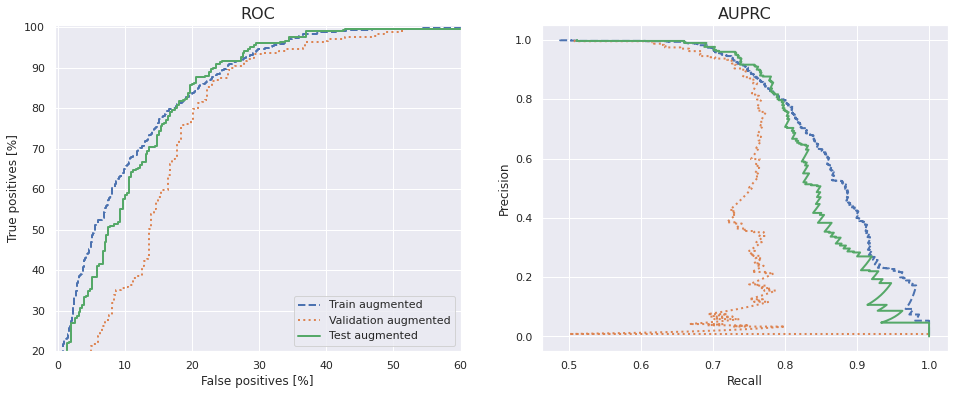
Plot the ROC and AUPRC

The same can be said about the ROC and AUPRC curves. The ROC might be slightly better than before though - achieving a 90% true positive rate on 23% false positives on the test set.

A more accurate way of comparing the performance of this model and the baseline would be to run many of each and compare the averages. So let's do that next.

Train and evaluate multiple models

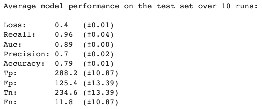
Let's train and evaluate 10 models with data augmentation. Use 50% dropout and train for 25 epochs each.

As displayed below, the standard deviation for each metric is lower than for the baseline model. This indicates that adding data augmentation and dropout seem to have a stabilising effect. Also, loss, recall, AUC and accuracy are all slightly higher indicating an overall better model. The precision is still fairly low though at 70% as before.

A common approach when working with limited datasets is to make use of pre-trained models. We will examine that next.

Pre-trained Xception model (Transfer Learning)

Transfer learning constitutes of using an already trained model and apply that on a different problem. The overall idea is that by pre-training a model on a large dataset the model is able to learn features that can be generalised to other domains. The larger and more comprehensive this dataset is the better the features the pre-trained model is able to learn, effectively acting as a generic model of the visual world, and the more useful can these learned features become in other computer vision problems.

We will be using an Xception architecture pre-trained on the Imagenet dataset - a dataset so large few researchers and engineers have the resources to train a model from scratch on. 1.2 million images divided into 1000 categories were used during pre-training, although, the dataset spans more than 14 million images.

The approach we will take is to build a model using the Xception architecture as convolutional base and add a densely connected classifier on top. Only the convolutional base has been trained on Imagenet before and it's these weights we will load into the model.

Load the Xception convolutional base

Load the Xception convolutional base and instantiate it with weights='imagenet'. Specifying include_top=False excludes the densely connected layer on top (we want to use our own). The reason for this is that the lower layers in the model have a tendency to contain more generalised mapping between the features and the target while the top layers tend to be more task specific.

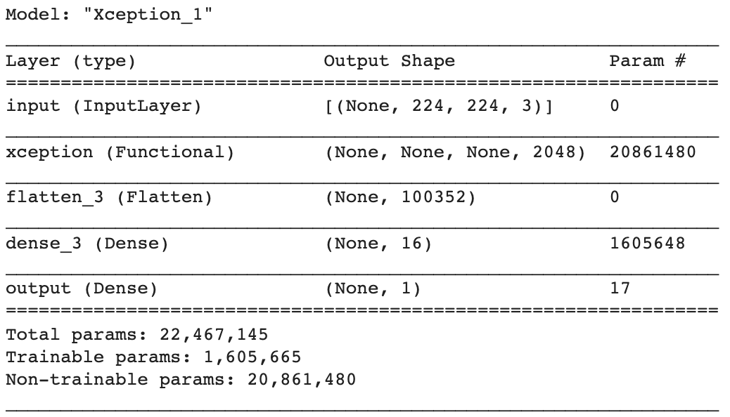
Running the code above instantiates the Xception convolutional base and outputs a (very long) architecture summary as shown below.

Note how large the Xception base above is with 14 blocks in total - each constitute of many layers. There's a total of 20,861,480 parameters, as compared to the baseline's 49,756 parameters. That's over 400 times more parameters!

Add a classifier on top and freeze the convolutional base

Apart from the Xception convolutional base added, building this model looks very similar to before.

Before compiling and training the model, it's very important to freeze the convolutional base. Freezing a layer or a set of layers means preserving the weights from being updated during training. If we don't do this, then the representations that were previously learned by the convolutional base will be modified during training and potentially destroyed. We can do that in Keras by setting the attribute trainable=False.

Above code block will output the following.

By compiling the model we store these changes. We also lower the learning rate to slow down the learning a bit.

After freezing the convolutional base, there should be significantly fewer trainable parameters as shown below.

Train the model

We set the model to train for 100 epochs while adjusting it to stop training if there's no improvement on validation AUC over 10 epochs.

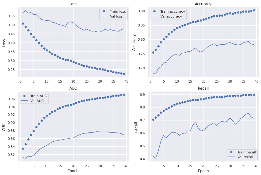
Check training history

When inspecting the metrics during training we note lower bias than with previous approaches. The accuracy, AUC and recall curves are reaching higher on the train set than before. The training loss also keeps decreasing indicating that the learning capacity of the model hasn't reached its limit yet. However, all four metrics stagnates on the validation set after around 25 epochs and gives us a model with high variance. This discrepancy in performance between the train and validation sets can be a result of a too small dataset. One of the best ways of dealing with high variance is normally to let the model train on more data.

Confusion matrix

Taking a look at the performance on the test set we note that it's roughly in par with previous models'. The major difference here though is higher precision, meaning that the model gets it right more frequently than before. There seem to have been a trade-off though; lower recall.

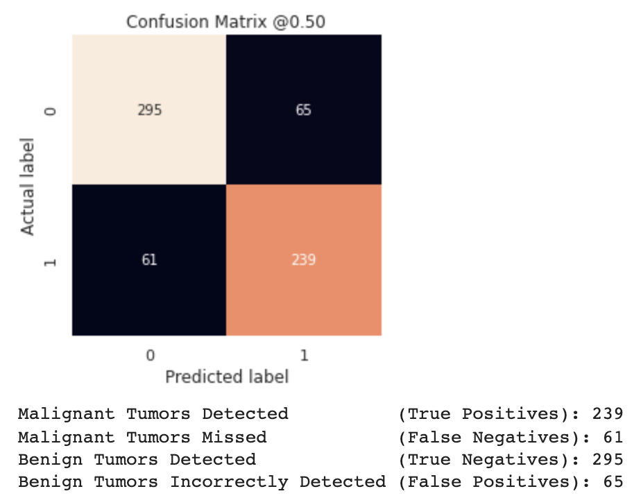
61 malignant tumors are missed by the model - a significant number and more than before. However, there are also considerable fewer incorrectly detected benign tumors (65).

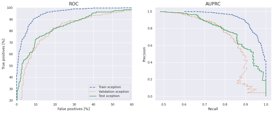
Plot the ROC and AUPRC

The ROC and AUPRC plots are displayed below and they confirm the high variance; a difference between the train set on one hand, and the validation and test sets on the other.

Train and evaluate multiple Xception models

Instantiate, train and evaluate multiple pre-trained Xception models.

Using a pre-trained Xception model do seem to decrease the standard deviation across most metrics as shown above. That's a good thing as we can then feel better about the model's performance at any given moment. We can also confirm a higher precision compared with before, while maintaining roughly the same accuracy and AUC. The higher precision has been traded for lower recall though. Importantly, the model also takes longer to train and uses more disc space than previous models (around 100MB).

Fine-tune the Xception model

It's often fruitful to fine-tune pre-trained models. However, as stated earlier, it's necessary to freeze the Xception convolutional base in order to be able to train the classifier on top. For the same reason, it's only possible to fine-tune the top layers of the convolutional base once the classifier on top has already been trained. If the classifier isn't already trained, the error signal propagating through the network during training will be so large that the previously learned weights will be destroyed. Moving forward, the steps for fine-tuning a pre-trained network are:

1. Add a custom network on top of an already-trained network.
2. Freeze the already-trained base network.
3. Train the added custom network.
4. Unfreeze some of the top layers in the base network.
5. Jointly train both these layers and the added custom network.

We have already implemented the first three steps. Let's move forward with unfreezing some of the last layers in the Xception convolutional base. Remember that the first layers learn more generic features while the later (or, further down) learn more specific to the task. The initial weights have been trained on Imagenet; a dataset with a lot of pictures on animals, nature and humans - which are quite different from cancer tumors. Transfer learning has proven successful across very diverse datasets, but in order to increase the probability of learning more tumor relevant features in the last few layers, we will unfreeze a larger chunk. In this particular case, let's choose to unfreeze all layers in block14; a total of 6 layers. Experimenting with unfreezing more blocks might be a good idea though.

Specify trainable layers

All layers in block14 will be unfrozen, as displayed below.

This results in the following model architecture.

By unfreezing the last 6 layers in block14 we have increased the number of trainable parameters from 1.6 million to around 6.4 million.

Tune and evaluate the Xception model

We will train the model with a very low learning rate to not risk destroying the weights already learned by the network. After around 17 minutes, the validation AUC stops improving and the training terminates.

The curves display similar characteristics as before with significant variance and fairly low bias. It's unclear whether fine-tuning has improved the performance by only looking at these plots though.

There seem to be little difference between the fine-tuned Xception model and the previous version where we only trained the custom classifier on top. In some cases we can expect a few percent of improvement though. The small differences even indicate that fine-tuning decreased model performance slightly. But again, this might be explained by random initiation during training and data loading and should rather be more thoroughly investigated by running multiple models and averaging their results. That is pretty computational expensive and will be left to future work though.

The ROC and AUPRC curves confirm high variance also for the fine-tuned model.

Summary

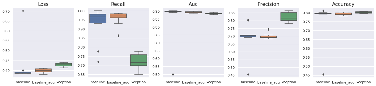
The plots below display the average loss, recall, AUC, precision and accuracy for the baseline, baseline with data augmentation and Xception with data augmentation over 10 runs on the test set. By only looking at the plots below it's not clear which model performs best. There are tradeoffs where higher recall and lower precision (the both baselines) are traded for lower recall but higher precision (Xception). All three models display similar AUC and accuracy. Adding data augmentation significantly decreases the standard deviation across all metrics and lead to more stable models.

In order to get a more holistic view of the models' performance, we should compare the metrics on the train and validation sets as well. As for the baseline and augmented baseline, the models reach their maximum learning capacity early on - meaning that there is little room for improvements even though we would add more data. However, the Xception model keeps improving on the training set even after the validation metrics have stagnated. The resulting high variance can often be treated by adding more data to the model with a resulting boost in performance.

Thus, if we are limited to current data, it might be better to go with the data augmented baseline as its performance is comparable to the larger Xception model, but is faster to train, takes less space on disk and is in general less complex. It's also more reliable than the baseline without augmented data. However, if there is a way to collect more data, the Xception model will likely do significantly better across most, if not all, metrics.

We conclude that it is possible to classify malignant from benign skin cancer using deep learning. Future work should start by collecting more data as it will likely yield the largest improvements.