What makes a Song Popular on Spotify?

My father compose music and was curious to know whether popular songs possess some typical characteristics. Let's see if we can find that out using common data science tools. My intuition is that shorter, vocal and more energetic songs are more popular among the general population. These are the kind of songs you hear most frequently when tuning into the radio or checking the top tracks of the month. Is it possible to prove this statistically? Moreover, is your music taste more in line with the general public's, or you've developed a unique taste of your own?

The dataset I will be using for the analysis can be downloaded here, while the column descriptions can be found at Spotify's developer page. The Jupyter notebook used for performing the analysis can be accessed in its fullest on GitHub here.

Initial data exploration

Load the data, decode the mode and popularity columns for ease of understanding, and delete two columns we're not interested in. Finally, display some statistics to make an initial verification that the data is okay.

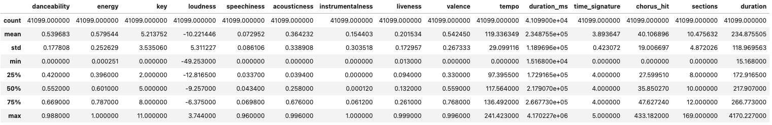
All columns seem to have reasonable range. Max duration (duration_ms) is very high at 4.17e6, but converted into something more comprehensible it's actually no more than 70 minutes (around 4000 seconds) - well within what's plausible for a song length. Many song attributes are normalised within the range [0, 1] (such as danceability, energy and instrumentalness).

Display what decades most songs are from, split on popularity and mode.

The data consist of most songs from the 60s and 70s. Major mode is more frequent than Minor mode.

Let's see what attributes are most correlated with popular songs by calculating the Pearson correlation coefficient between each feature and the popularity. This can then be displayed in something referred to as a correlation matrix.

Pearson Correlation Matrix

In order to facilitate interpretation of the correlation matrix, I will rearrange the column order so popularity ends up in the first position. Some columns need to be converted to numerical as well. Below is the resulting matrix.

The attributes that are most correlated with song popularity, when considering both popular and unpopular songs, are:

• Instrumentalness (-0.41)
• Danceability (0.35)
• Loudness (0.29)
• Valence (0.25) and Acousticness (-0.25)
• Energy (0.20)

Attributes such as decade, duration, tempo, liveness and speechiness have only minor impact.

We can additionally confirm this using A/B tests. We won't cover all but will instead focus on some few in each group; highly and minor correlated. For the purpose of this article we choose to test instrumentalness, danceability and energy among the highly correlated attributes and duration and speechiness among the features with low correlation.

Since we will conduct the analysis based on popular and unpopular songs, we will split the data into these two groups.

With around 20.000 songs in each group, the dataset is more than large enough for hypothesis testing.

Instrumentalness

Instrumentalness was highly negatively correlated with song popularity. This means that songs that are popular have in general lower instrumentalness. This makes intuitive sense as most songs you hear on the popular radio stations are not instrumental. Let's very this statistically using an A/B test.

Since we have more than 2,000 samples, we will use Jarque-Bera and Scipy's Normaltest to test for normality.

Plot instrumentalness by popularity using a histogram. Then calculate skewness and kurtosis and test for normality.

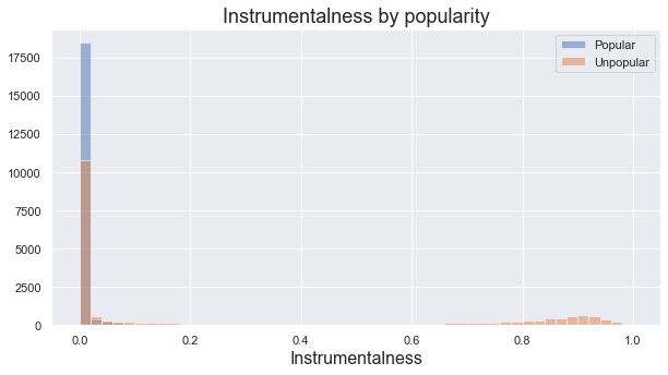
Both skewness and kurtosis are above the threshold of ±3 for popular songs which indicates non-normality. Jarque-Bera and Normaltest as well as a visual inspection confirms this. Although unpopular songs have acceptable values, we choose Kruskal-Wallis test for testing the null hypothesis.

State the null and alternative hypothesis

• The null hypothesis is that there is no significant difference, on average, in Instrumentalness between popular and unpopular songs.
• The alternative hypothesis is that there is a significant difference, on average, in Instrumentalness between popular and unpopular songs.

Test the null hypothesis and visualise the results.

This results in a t-statistics of 7265.83 and a p-value of 0.0. We can even choose a confidence level of 99% for the confidence interval due to the low p-value. The high t-statistics indicate a large difference between the groups. Let's calculate the confidence interval by wrapping corresponding logic in a function.

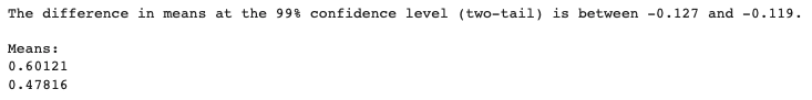
Which results in the following output:

We reject the null. There is a significant difference in means between the two groups. With 99% confidence, popular songs have between 0.24 and 0.25 points lower nstrumentalness than unpopular songs.

It can be difficult to imagine this difference in means by just looking at the numbers. Below plot makes this slightly clearer.

Visually the difference is clear, with means at around 0.03 and 0.28. Unpopular songs are on average far more instrumental (around 8 times more) than those that are popular.

Danceability

Through the correlation matrix earlier, we saw that danceability is positively correlated with song popularity. This means that popular songs tend to be more danceable. This makes sense based on the songs that seem to be most frequently played on mainstream radio stations.

Similar to before, display danceability by popularity using a histogram.

Both distributions seem to be close to normally distributed by a visual inspection.

Both skewness and kurtosis are well below the threshold of ±3 for normality, while the test statistics is very close to 1. Great! We can more forward with an independent t-test.

State the null and alternative hypothesis

• The null hypothesis is that there is no significant difference, on average, in Danceability between popular and unpopular songs.
• The alternative hypothesis is that there is a significant difference, on average, in Danceability between popular and unpopular songs.

Test the null hypothesis and visualise the results

We get a t-statistics of 74.76 and a p-value of 0.0. Since the p-value is so low, we can go with a 99% confidence level when calculating the confidence interval.

We reject the null. With 99% confidence, popular songs have on average between 0.12 and 0.13 higher danceability scores than unpopular songs. This is equivalent to a difference of around 25%.

We can visually see that the average danceability for popular songs is significantly higher (at 0.60) compared with unpopular (0.48) songs. Note the small confidence intervals (vertical lines through the dots which you barely see) - they're a result of the large sample size which allows us to calculate the difference more accurately.

Energy

The energy level had a fairly high positive correlation among popular songs. This means that popular songs have in general higher energy level than those that are not. Plotting the distribution for energy level by popularity on a histogram yields the following plot:

Calculating skewness, kurtosis and testing for normality results in the following.

A visual inspection seem to indicate that the most energetic songs are unpopular (energy level at or close to 1). Popular songs are still clustered in the higher end with most energetic songs scoring around 0.5 and 0.8. Energy level among popular songs is fairly normally distributed, while that doesn't seem to be the case for unpopular songs.

Although skewness and kurtosis indicate that both distributions are normal, the unpopular songs visuals are not convincing. We will thus go with Kruskal-Wallis non-parametric test to be on the safe side. The sample size is with good margin large enough.

State the null and alternative hypothesis

• The null hypothesis is that there is no significant difference, on average, in Energy level between popular and unpopular songs.
• The alternative hypothesis is that there is a significant difference, on average, in Energy level between popular and unpopular songs.

Test the null hypothesis and visualise the results

We get a t-statistics of 904.27 and a very small p-value of 1.16e-198. The confidence interval is displayed as follows:

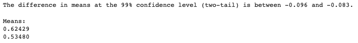
We reject the null. With 99% confidence, popular songs have on average between 0.08 and 0.1 higher energy level units than unpopular songs. A difference of around 17%.

Above point plot visually displays how the average energy level for popular songs (0.62) is significantly higher than for unpopular songs (0.53).

Duration

Duration had a very low negative correlation with song popularity in our initial analysis.

Start by plotting the distribution. Out of the around 40k songs in the dataset, only 134 are longer than 1,000 seconds. This results in a very long right tail (the longest song is around 70 minutes, or over 4,000 seconds). By limiting the x-axis to 1,000 seconds, it will be easier to interpret the plot. The t-test will be applied on all songs though.

Skewness, kurtosis and a visual inspection all indicate that neither of the distributions are normal.

State the null and alternative hypothesis

• The null hypothesis is that there is no significant difference, on average, in Duration between popular and unpopular songs.
• The alternative hypothesis is that there is a significant difference, on average, in Duration between popular and unpopular songs.

Test the null hypothesis and visualise the results

We use the Kruskal-Wallis test to test the null and get a t-statistics of 18.98 and p-value of 1.32e-05.

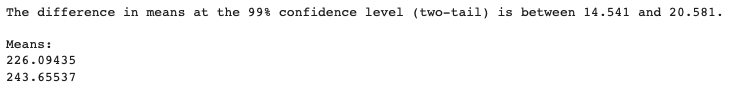
We reject the null. There is a significant difference in duration between popular and unpopular songs. With 99% confidence, popular songs are on average between 15 and 21 seconds shorter than unpopular songs.

This is not much, but I still find it reasonable that popular songs are at least slightly shorter than unpopular songs, on average. Few songs that are played on mainstream media platforms are very long. Let's visually display this difference below.

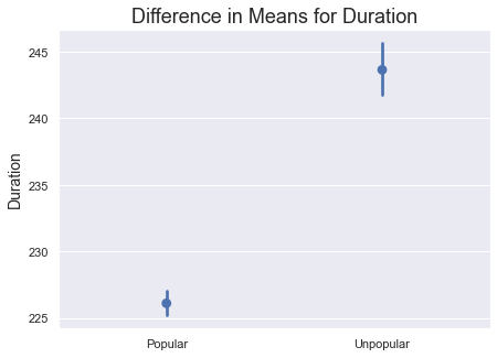
We initially found a weak negative correlation for song Duration using a correlation matrix. The A/B test verifies these results by confirming that there is a difference. However, the difference is quite small at around 8%.

Speechiness

Lastly, we will run an A/B test on Speechiness. Speechiness had a very weak negative correlation in our initial analysis. As before, plot the distribution to get a general feeling for the data.

There is no clear visual difference between popular and unpopular songs. They all compose of little speech. It seems like speech-rich content such as audio books and podcasts have been excluded from the dataset during data collection.

None of the distributions seem normal by a visual inspection. Both skewness and kurtosis suggest this as well. We will thus use Kruskal-Wallis to test the null hypothesis.

State the null and alternative hypothesis

• The null hypothesis is that there is no significant difference, on average, in Speechiness between popular and unpopular songs.
• The alternative hypothesis is that there is a significant difference, on average, in Speechiness between popular and unpopular songs.

Test the null hypothesis and visualise the results

We end up with a t-statistics of 697.39 and p-value of 1.10e-153.

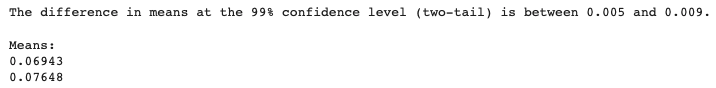
We reject the null. With 99% confidence, popular songs have on average between 0.005 and 0.009 lower speechiness score compared with unpopular songs. Although significant, the difference is quite small at around 10%.

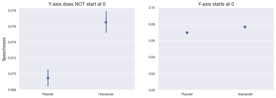
The left plot, which is using the default settings and a truncated y-axis, indicate a very large difference between the two distributions. The right plot, with a y-axis starting at 0, doesn't play tricks on us like that. It's important to be aware of small details like this when plotting the difference between two groups. The statistical test suggested a small difference - and this should be reflected in the visuals as well.

Conclusions

We've identified several attributes that differ between popular and unpopular songs. With high certainty and fairly large differences, Instrumentalness, Danceability and Energy level are significantly different between the two groups. The difference in both Duration and Speechiness were statistically significant but fairly small.

There are several caveats regarding the dataset. We don't know under what assumptions it was collected or whether it's representative for songs in general. It contains roughly as many popular as unpopular songs (20k) while it's fair to assume that there are more unpopular than popular songs on the market. We don't know exactly what defines a song as popular. Perhaps the definition is too loose or too restricted. The dataset contain only songs on Spotify, and although Spotify is a leader on the market, it may not represent popular songs on other platforms and in society in general.

Nevertheless, based on the data we've used, if you feel that most of the songs you're listening to are more danceable than not, have high energy levels and are most often not instrumental - then there's a chance your music would be popular among many others. On the other hand, if you don't recognise yourself listening to this kind of music, you might have a more unique taste. 🙂